Getting ready
Task 1
Create an R project for solving this Exercise Sheet.
Task 2
Download the csv-file SSRC_data.csv and the R script SSRC_C5_template.R and put it in the R project folder you created in Task 1.
Task 3
Open the SSRC_C5_template.R R Script.
Task 4
Load the tidyverse package.
# Load tidyverse package
library("tidyverse")
Task 5
Use the read.csv() command to load the SSRC data into R and call the respective data object SSRC_data.
# Load the dataset
SSRC_data <- read.csv("SSRC_data.csv")
Task 6
Get a first impression of the dataset by checking out the dataset using the str() command.
# Check out the dataset
str(SSRC_data)
'data.frame': 1000 obs. of 5 variables:
$ age : int 64 59 39 30 49 37 33 44 27 55 ...
$ gender : chr "male" "female" "female" "female" ...
$ education_level : chr "medium" "low" "high" "high" ...
$ physical_activity_level: chr "low" "medium" "low" "low" ...
$ bmi : num 27.9 27.5 27.4 24.2 23.9 30.7 25.1 30.3 18.5 30.2 ...Task 7
Transform the three categorical variables in the dataset into factor variables. Make sure that the levels of the physical_activity_level and education_level variables are ordered in a reasonable way. (You learned how to do that in chapter 2)
# Transform into factor variables
SSRC_data <- mutate(SSRC_data, gender = as.factor(gender),
                               education_level = as.factor(education_level),
                               physical_activity_level = as.factor(physical_activity_level))

# Order education_level and physical_activity_level in a reasonable way
SSRC_data <- SSRC_data %>%
              mutate(education_level = fct_relevel(education_level, c("low", "medium", "high"))) %>%
              mutate(physical_activity_level = fct_relevel(physical_activity_level, c("low", "medium", "high")))

# Check whether it worked out
levels(SSRC_data$education_level)
[1] "low" "medium" "high" levels(SSRC_data$physical_activity_level)[1] "low" "medium" "high" Linear Regression
Task 8
Analyze the relationship between age and bmi by fitting a linear regression model with the variable bmi as dependent variable and age as independent variable. Call this model lm_mod_restricted. Use the summary() command to check out the results.
# Estimate the model
lm_mod_restricted <- lm(bmi ~ age , data = SSRC_data)

# Check out model results
summary(lm_mod_restricted)
Call:
lm(formula = bmi ~ age, data = SSRC_data)

Residuals:
     Min       1Q   Median       3Q      Max
-10.5254  -2.8796  -0.4681   2.1459  28.2083

Coefficients:
            Estimate Std. Error t value Pr(>|t|)
(Intercept) 21.66782    0.50240   43.13   <2e-16 ***
age          0.10675    0.01013   10.54   <2e-16 ***
---
Signif. codes:  0 '***' 0.001 '**' 0.01 '*' 0.05 '.' 0.1 ' ' 1

Residual standard error: 4.338 on 998 degrees of freedom
Multiple R-squared:  0.1002,    Adjusted R-squared:  0.09931
F-statistic: 111.1 on 1 and 998 DF,  p-value: < 2.2e-16
Task 9
Estimate a linear regression model with bmi as dependent variable and all other variables in the SSRC data set as independent variables. Call this model lm_mod_full. Use the summary() command to check out the results.
# Estimate the model
lm_mod_full <- lm(bmi ~ age + gender + education_level + physical_activity_level, data = SSRC_data)

# Check out model results
summary(lm_mod_full)
Call:
lm(formula = bmi ~ age + gender + education_level + physical_activity_level,
    data = SSRC_data)

Residuals:
     Min       1Q   Median       3Q      Max
-12.0180  -2.6923  -0.5798   2.0490  28.4287

Coefficients:
                              Estimate Std. Error t value Pr(>|t|)
(Intercept)                   23.05859    0.65008  35.470  < 2e-16
age                            0.09195    0.01043   8.820  < 2e-16
gendermale                     0.88613    0.27589   3.212  0.00136
education_levelmedium         -0.81952    0.37033  -2.213  0.02713
education_levelhigh           -1.78693    0.40766  -4.383 1.29e-05
physical_activity_levelmedium -0.56293    0.33108  -1.700  0.08939
physical_activity_levelhigh   -0.22907    0.37725  -0.607  0.54385

(Intercept)                   ***
age                           ***
gendermale                    **
education_levelmedium         *
education_levelhigh           ***
physical_activity_levelmedium .
physical_activity_levelhigh
---
Signif. codes:  0 '***' 0.001 '**' 0.01 '*' 0.05 '.' 0.1 ' ' 1

Residual standard error: 4.283 on 993 degrees of freedom
Multiple R-squared:  0.1271,    Adjusted R-squared:  0.1218
F-statistic:  24.1 on 6 and 993 DF,  p-value: < 2.2e-16
Fitted Values and Residuals
Task 10
Use the lm_mod_full model you just fitted in task 9 to add the fitted bmi values to the SSRC dataset. Call this new variable bmi_fitted. Use the str() command to check out whether it worked.
# Add fitted bmi values to SSRC dataset
SSRC_data$bmi_fitted <- lm_mod_full$fitted.values

# Check out whether it worked
str(SSRC_data)
'data.frame': 1000 obs. of 6 variables:
$ age : int 64 59 39 30 49 37 33 44 27 55 ...
$ gender : Factor w/ 2 levels "female","male": 2 1 1 1 2 2 2 2 1 1 ...
$ education_level : Factor w/ 3 levels "low","medium",..: 2 1 3 3 2 2 3 2 3 2 ...
$ physical_activity_level: Factor w/ 3 levels "low","medium",..: 1 2 1 1 1 2 1 3 2 1 ...
$ bmi : num 27.9 27.5 27.4 24.2 23.9 30.7 25.1 30.3 18.5 30.2 ...
$ bmi_fitted : num 29 27.9 24.9 24 27.6 ...Task 11
Calculate the residuals by substracting the fitted values from the true observed bmi values and add this residuals variable to the SSRC dataset. Check out whether it worked.
# Calculate residuals
SSRC_data <- mutate(SSRC_data, residuals = bmi - bmi_fitted)

# Check out whether it worked
str(SSRC_data)
'data.frame': 1000 obs. of 7 variables:
$ age : int 64 59 39 30 49 37 33 44 27 55 ...
$ gender : Factor w/ 2 levels "female","male": 2 1 1 1 2 2 2 2 1 1 ...
$ education_level : Factor w/ 3 levels "low","medium",..: 2 1 3 3 2 2 3 2 3 2 ...
$ physical_activity_level: Factor w/ 3 levels "low","medium",..: 1 2 1 1 1 2 1 3 2 1 ...
$ bmi : num 27.9 27.5 27.4 24.2 23.9 30.7 25.1 30.3 18.5 30.2 ...
$ bmi_fitted : num 29 27.9 24.9 24 27.6 ...
$ residuals : num -1.11 -0.421 2.542 0.17 -3.731 ...Task 12
Analyze the distribution of the residuals variable you created in task 11 with a histogram and a density plot.
# Histogram
ggplot(data = SSRC_data) +
  geom_histogram(mapping = aes(x = residuals))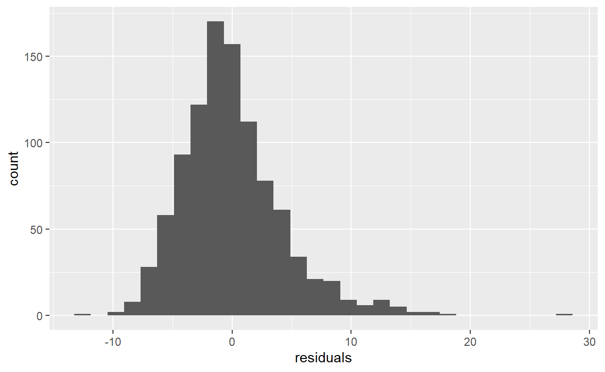
# Density Plot
ggplot(data = SSRC_data) +
  geom_density(mapping = aes(x = residuals))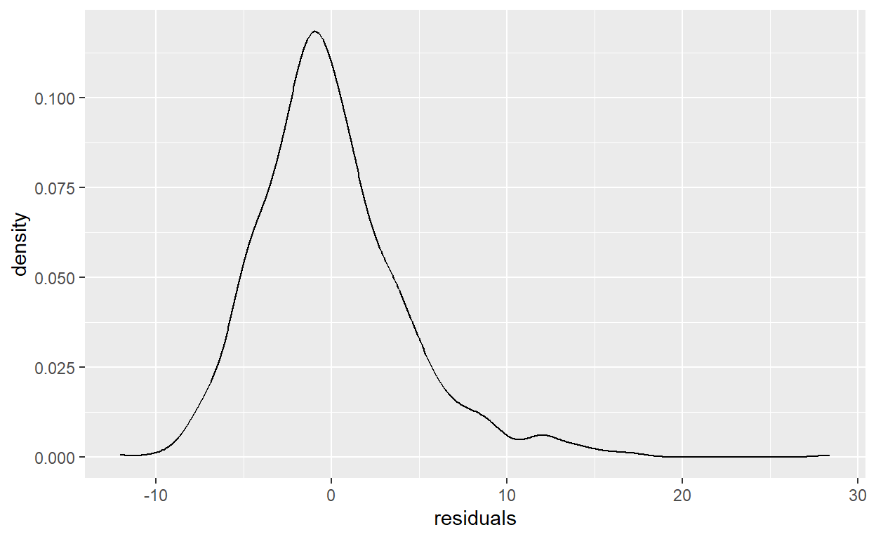
Prediction
Task 13
Create a data frame with two observations and the four variables: age, gender, education_level and physical_activity_level. The first observation is a female person of age 28 who features both a high level of education and a high level of physical activity. The second observation is a male person of age 59 who features a medium level of education and a low level of physical activity. Call this data frame SSRC_data_new.
# Create data frame
SSRC_data_new <- data.frame(age = c(28, 59),
                            gender = c("female", "male"),
                            education_level = c("high", "medium"),
                            physical_activity_level = c("high", "low"))
Task 14
Use the lm_mod_full model to predict the bmi for the two new observations described in Task 13.
# Predict bmi for new observations
predict(object = lm_mod_full,
        newdata = SSRC_data_new)
1 2
23.61717 28.55019 Extracting Coefficients
Task 15
Extract the beta coefficients for the age variable from the lm_mod_full and the lm_mod_restricted model objects. Combine them in data frame that displays the two age coefficients nicely next to each other and where the columns are called full_model and restricted_model. Call this data frame age_coefficients and check it out after creating it.
# Extract coefficient from the full model
matrix_coef_full <- summary(lm_mod_full)$coefficients
age_coef_full <- matrix_coef_full[2,1]

# Extract coefficient from the restricted model
matrix_coef_restricted <- summary(lm_mod_restricted)$coefficients
age_coef_restricted <- matrix_coef_restricted[2,1]

# Create data frame
age_coefficients <- data.frame(full_model = c(age_coef_full),
                               restricted_model = c(age_coef_restricted))

# Check out the created data frame
age_coefficients
full_model restricted_model
1 0.09194905 0.1067474Logistic Regression
Task 16
Create an indicator variable that equals one if the bmi of a person is larger or equal to 30 and zero otherwise. Add this variable to the SSRC dataset and call it obesity. (You can use the mutate() command in combination with the ifelse() command to do this in one line of code)
Task 17
Fit a logistic regression model with the obesity variable as dependent variable and age, gender, education_level and physical_activity_level as independent variables. Call this model logit_mod. Use the summary() command to check out the results.
# Fit logistic regression model
logit_mod <- glm(obesity ~ age  + gender + education_level + physical_activity_level,
                 data = SSRC_data,
                 family = binomial)

# Check out the results
summary(logit_mod)
Call:
glm(formula = obesity ~ age + gender + education_level + physical_activity_level,
    family = binomial, data = SSRC_data)

Deviance Residuals:
    Min       1Q   Median       3Q      Max
-1.0486  -0.7194  -0.5695  -0.4182   2.2982

Coefficients:
                               Estimate Std. Error z value Pr(>|z|)
(Intercept)                   -2.459804   0.393658  -6.249 4.14e-10
age                            0.029040   0.006326   4.591 4.42e-06
gendermale                    -0.005055   0.164956  -0.031  0.97555
education_levelmedium         -0.189523   0.201150  -0.942  0.34609
education_levelhigh           -0.700715   0.243259  -2.881  0.00397
physical_activity_levelmedium -0.178425   0.203634  -0.876  0.38092
physical_activity_levelhigh   -0.161307   0.233540  -0.691  0.48975

(Intercept)                   ***
age                           ***
gendermale
education_levelmedium
education_levelhigh           **
physical_activity_levelmedium
physical_activity_levelhigh
---
Signif. codes:  0 '***' 0.001 '**' 0.01 '*' 0.05 '.' 0.1 ' ' 1

(Dispersion parameter for binomial family taken to be 1)

    Null deviance: 1006.3  on 999  degrees of freedom
Residual deviance:  962.4  on 993  degrees of freedom
AIC: 976.4

Number of Fisher Scoring iterations: 4
Task 18
Predict the probability that the two new observations described in Task 13 are obese. You can reuse the SSRC_data_new dataframe. You can also use the type option of the predict() command to get the predicted probabilities directly. Just set type equal to “response”.
# Calculate the obesity probability for the two new observations
predict(object = logit_mod,
        newdata = SSRC_data_new,
        type = "response")
1 2
0.07525069 0.28069762