Data preparation
Load Packages
Load and rename datasets
### Load datasets and give them intuitive names

# Dataset with cvd event data
data_cvd_event <- read.csv("SSRC_dataset_case_study_1.csv")

# Dataset with portfolio data
data_portfolio <- read.csv("SSRC_dataset_case_study_2.csv")

### Check out structure of the two datasets
str(data_cvd_event)
'data.frame': 10000 obs. of 7 variables:
$ v1: int 61 64 42 73 51 32 55 55 44 55 ...
$ v2: int 1 0 1 0 1 1 1 1 1 1 ...
$ v3: int 0 1 0 0 0 0 0 0 0 0 ...
$ v4: num 30.1 26 30.4 26.9 27.4 20.7 46.4 22.6 26.3 38.6 ...
$ v5: num 126 124 104 127 117 ...
$ v6: num 62.8 73.5 61.6 70.1 81.3 ...
$ v7: int 0 1 0 0 0 0 0 0 0 0 ...str(data_portfolio)'data.frame': 5000 obs. of 6 variables:
$ v1: int 24 56 35 34 39 34 49 41 26 29 ...
$ v2: int 0 1 0 1 0 0 1 0 0 1 ...
$ v3: int 0 0 0 1 0 1 0 0 0 1 ...
$ v4: num 23.9 31.1 27.4 29.4 26.6 26.5 24.4 33.1 27 27.7 ...
$ v5: num 120 121 118 126 137 ...
$ v6: num 77.6 75.3 77.2 79.9 90.8 80 83.7 91.1 59.7 85.1 ...Rename variables
### Assign intuitive and self-explanatory names to the variables

# CVD event dataset
data_cvd_event <- rename(data_cvd_event, age = v1,
                                         gender = v2,
                                         smoking = v3,
                                         bmi = v4,
                                         systolic_bp = v5,
                                         diastolic_bp = v6,
                                         cvd_event = v7)

str(data_cvd_event)
'data.frame': 10000 obs. of 7 variables:
$ age : int 61 64 42 73 51 32 55 55 44 55 ...
$ gender : int 1 0 1 0 1 1 1 1 1 1 ...
$ smoking : int 0 1 0 0 0 0 0 0 0 0 ...
$ bmi : num 30.1 26 30.4 26.9 27.4 20.7 46.4 22.6 26.3 38.6 ...
$ systolic_bp : num 126 124 104 127 117 ...
$ diastolic_bp: num 62.8 73.5 61.6 70.1 81.3 ...
$ cvd_event : int 0 1 0 0 0 0 0 0 0 0 ...# Portfolio dataset
data_portfolio <- rename(data_portfolio, age = v1,
gender = v2,
smoking = v3,
bmi = v4,
systolic_bp = v5,
diastolic_bp = v6)
str(data_portfolio)'data.frame': 5000 obs. of 6 variables:
$ age : int 24 56 35 34 39 34 49 41 26 29 ...
$ gender : int 0 1 0 1 0 0 1 0 0 1 ...
$ smoking : int 0 0 0 1 0 1 0 0 0 1 ...
$ bmi : num 23.9 31.1 27.4 29.4 26.6 26.5 24.4 33.1 27 27.7 ...
$ systolic_bp : num 120 121 118 126 137 ...
$ diastolic_bp: num 77.6 75.3 77.2 79.9 90.8 80 83.7 91.1 59.7 85.1 ...Create factors and rename levels
# CVD event dataset
data_cvd_event <- data_cvd_event %>%
                        mutate(gender = as.factor(gender)) %>%
                        mutate(gender = fct_recode(gender, "male" = "0", "female" = "1")) %>%
                        mutate(smoking = as.factor(smoking)) %>%
                        mutate(smoking = fct_recode(smoking, "no" = "0", "yes" = "1")) %>%
                        mutate(cvd_event = as.factor(cvd_event)) %>%
                        mutate(cvd_event = fct_recode(cvd_event, "no" = "0", "yes" = "1"))

head(data_cvd_event)
age gender smoking bmi systolic_bp diastolic_bp cvd_event
1 61 female no 30.1 126.3 62.8 no
2 64 male yes 26.0 123.6 73.5 yes
3 42 female no 30.4 104.1 61.6 no
4 73 male no 26.9 127.2 70.1 no
5 51 female no 27.4 117.0 81.3 no
6 32 female no 20.7 107.4 76.4 no# Portfolio dataset
data_portfolio <- data_portfolio %>%
mutate(gender = as.factor(gender)) %>%
mutate(gender = fct_recode(gender, "male" = "0", "female" = "1")) %>%
mutate(smoking = as.factor(smoking)) %>%
mutate(smoking = fct_recode(smoking, "no" = "0", "yes" = "1"))
head(data_portfolio) age gender smoking bmi systolic_bp diastolic_bp
1 24 male no 23.9 120.5 77.6
2 56 female no 31.1 120.9 75.3
3 35 male no 27.4 118.2 77.2
4 34 female yes 29.4 126.4 79.9
5 39 male no 26.6 137.0 90.8
6 34 male yes 26.5 130.5 80.0Create hypertension variable
### Create hypertension indicator

# CVD event dataset
 data_cvd_event <- data_cvd_event %>%
                          mutate(hypertension = if_else(systolic_bp >= 140 | diastolic_bp >= 90, "yes", "no")) %>%
                          mutate(hypertension = as.factor(hypertension)) %>%
                          mutate(hypertension = fct_relevel(hypertension, c("no", "yes")))
head(data_cvd_event)
age gender smoking bmi systolic_bp diastolic_bp cvd_event
1 61 female no 30.1 126.3 62.8 no
2 64 male yes 26.0 123.6 73.5 yes
3 42 female no 30.4 104.1 61.6 no
4 73 male no 26.9 127.2 70.1 no
5 51 female no 27.4 117.0 81.3 no
6 32 female no 20.7 107.4 76.4 no
hypertension
1 no
2 no
3 no
4 no
5 no
6 no# Portfolio dataset
data_portfolio <- data_portfolio %>%
mutate(hypertension = if_else(systolic_bp >= 140 | diastolic_bp >= 90, "yes", "no")) %>%
mutate(hypertension = as.factor(hypertension)) %>%
mutate(hypertension = fct_relevel(hypertension, c("no", "yes")))
head(data_portfolio) age gender smoking bmi systolic_bp diastolic_bp hypertension
1 24 male no 23.9 120.5 77.6 no
2 56 female no 31.1 120.9 75.3 no
3 35 male no 27.4 118.2 77.2 no
4 34 female yes 29.4 126.4 79.9 no
5 39 male no 26.6 137.0 90.8 yes
6 34 male yes 26.5 130.5 80.0 noData exploration
Variation
Age
# Summary statistics
summary(data_cvd_event$age)
Min. 1st Qu. Median Mean 3rd Qu. Max.
22.00 37.00 48.00 48.27 59.00 77.00 # Density plot
ggplot(data = data_cvd_event) +
geom_density(mapping = aes(x = age))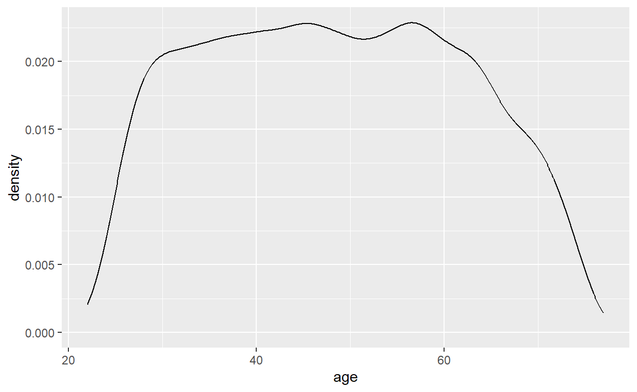
Gender
  male female
0.4967 0.5033 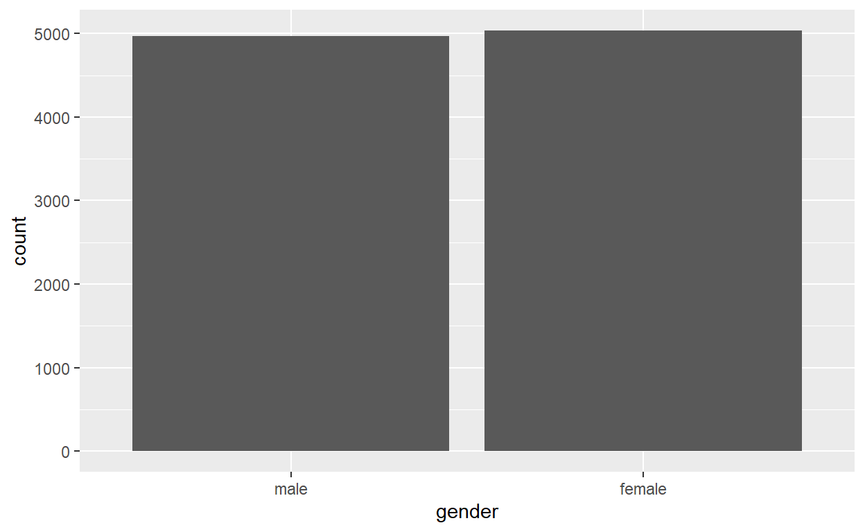
Smoking Status
    no    yes
0.7381 0.2619 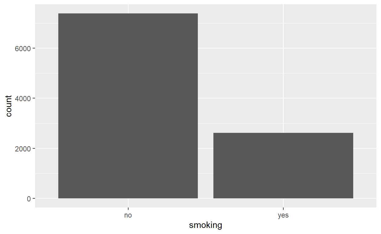
BMI
# Summary statistics
summary(data_cvd_event$bmi)
Min. 1st Qu. Median Mean 3rd Qu. Max.
16.00 23.70 26.30 26.77 29.20 57.00 # Density plot
ggplot(data = data_cvd_event, mapping = aes(x = bmi)) +
geom_density()
Hypertension Status
    no    yes
0.6801 0.3199 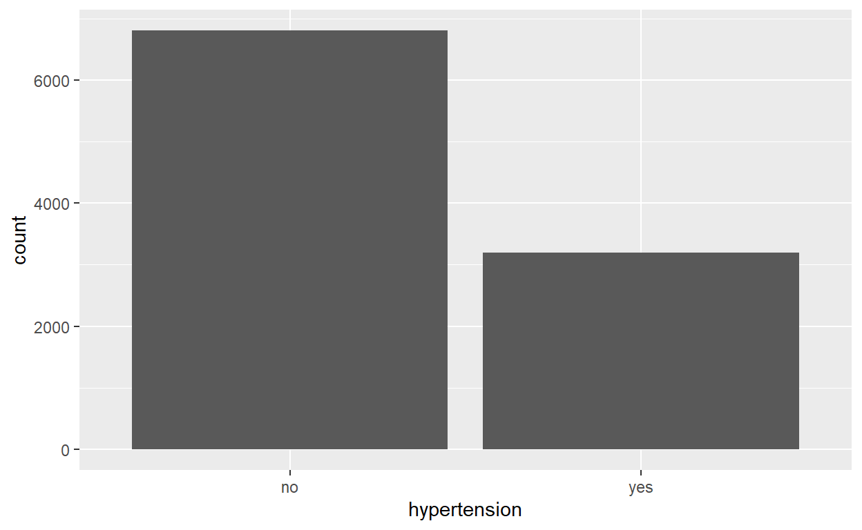
CVD event indicator
    no    yes
0.9283 0.0717 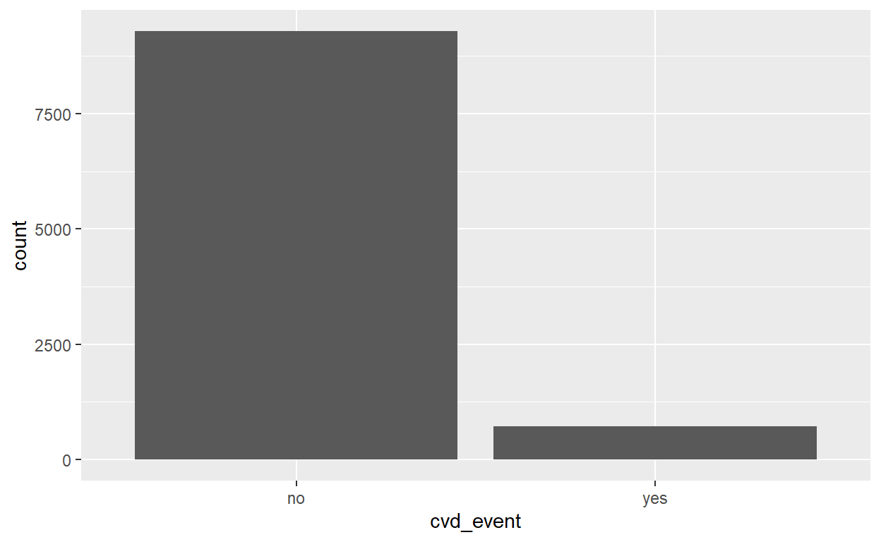
Covariation
CVD and age
# Grouped summary
data_cvd_event %>%
  group_by(cvd_event) %>%
  summarize(mean_age = mean(age), median_age = median(age))
# A tibble: 2 × 3
cvd_event mean_age median_age
<fct> <dbl> <int>
1 no 47.2 47
2 yes 62.3 64# Boxplot
ggplot(data = data_cvd_event) +
geom_boxplot(mapping = aes( x = age, y = cvd_event)) +
coord_flip()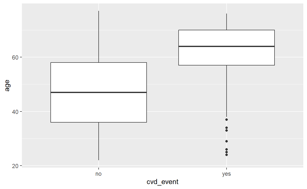
CVD and gender
             no    yes
  male   0.4513 0.0454
  female 0.4770 0.0263
CVD and bmi
# Grouped summary
data_cvd_event %>%
  group_by(cvd_event) %>%
  summarize(mean_bmi = mean(bmi), median_bmi = median(bmi))
# A tibble: 2 × 3
cvd_event mean_bmi median_bmi
<fct> <dbl> <dbl>
1 no 26.6 26.2
2 yes 28.7 28 # Boxplot
ggplot(data = data_cvd_event, mapping = aes(x = bmi, y = cvd_event)) +
geom_boxplot() +
coord_flip()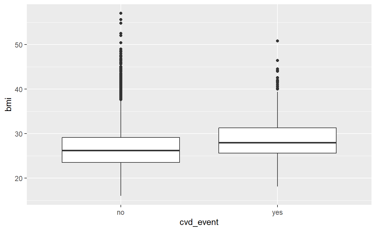
Regression analysis
# Estimate logit model
logit_mod <- glm(cvd_event ~ age + gender + smoking + bmi + hypertension,
                 family = "binomial",
                 data = data_cvd_event)

# Show results
summary(logit_mod)
Call:
glm(formula = cvd_event ~ age + gender + smoking + bmi + hypertension,
    family = "binomial", data = data_cvd_event)

Deviance Residuals:
    Min       1Q   Median       3Q      Max
-1.4059  -0.3883  -0.2031  -0.1027   3.6937

Coefficients:
                 Estimate Std. Error z value Pr(>|z|)
(Intercept)     -9.958050   0.390190 -25.521  < 2e-16 ***
age              0.107249   0.004554  23.548  < 2e-16 ***
genderfemale    -0.525380   0.087202  -6.025 1.69e-09 ***
smokingyes       0.821408   0.100528   8.171 3.06e-16 ***
bmi              0.042202   0.009698   4.352 1.35e-05 ***
hypertensionyes  0.559488   0.086876   6.440 1.19e-10 ***
---
Signif. codes:  0 '***' 0.001 '**' 0.01 '*' 0.05 '.' 0.1 ' ' 1

(Dispersion parameter for binomial family taken to be 1)

    Null deviance: 5160.3  on 9999  degrees of freedom
Residual deviance: 4040.7  on 9994  degrees of freedom
AIC: 4052.7

Number of Fisher Scoring iterations: 7
Identification of high risks
### Predict cvd event probabilities for the portfolio datases
data_portfolio <- mutate(data_portfolio, cvd_risk = predict(logit_mod, newdata = data_portfolio, type = "response"))


### Distribution of cvd_risk
# Summary statistics
summary(data_portfolio$cvd_risk)
Min. 1st Qu. Median Mean 3rd Qu. Max.
0.0008237 0.0083777 0.0307492 0.0756245 0.1041549 0.6879710 # Density plot
ggplot(data = data_portfolio, mapping = aes(x = cvd_risk)) +
geom_density()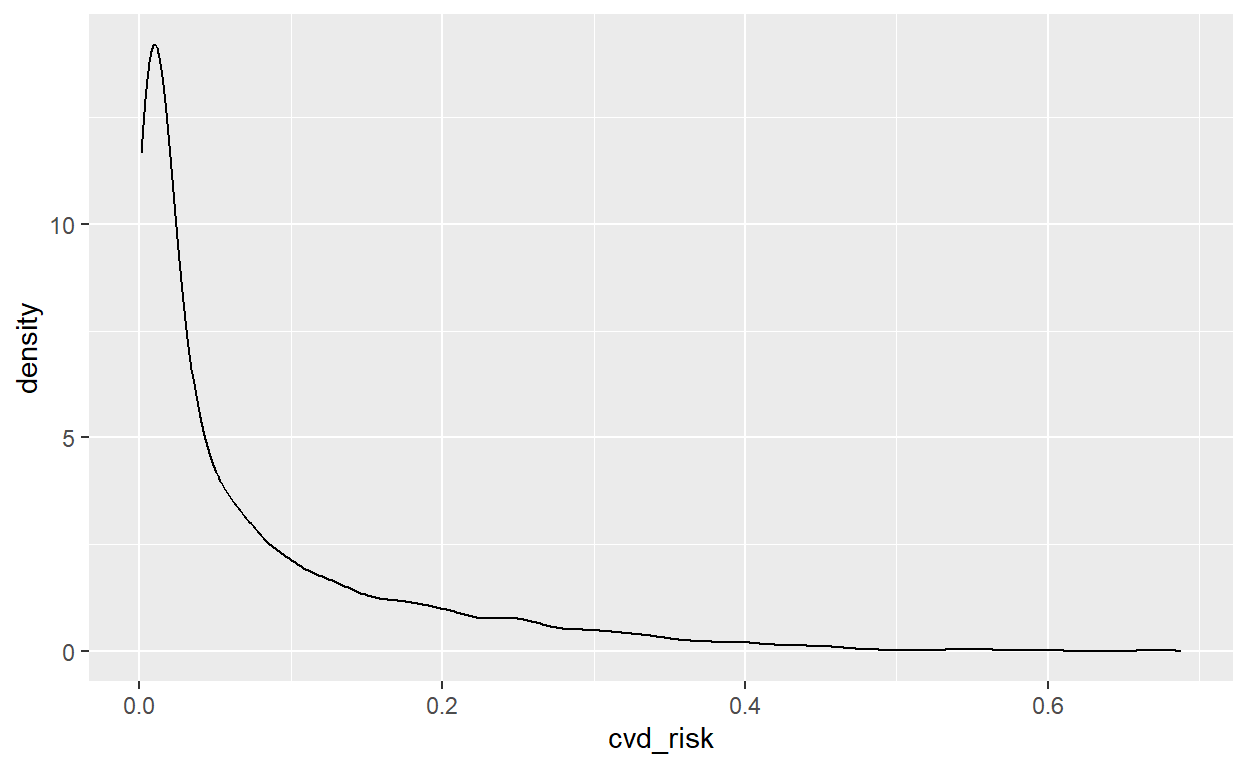
### Create high risk indicator variable
data_portfolio <- mutate(data_portfolio, high_cvd_risk = if_else(cvd_risk > 0.1, "yes", "no"))

table(data_portfolio$high_cvd_risk)
  no  yes
3709 1291
    no    yes
0.7418 0.2582
Expected number of events
### Calculate the expected number of cvd events in the upcoming 10 years in the portfolio
exp_number_cvd_events <- sum(data_portfolio$cvd_risk)

exp_number_cvd_events
[1] 378.1226### Create vector with 1000 estimates for the expected numbers of cvd events in the portfolio
exp_number_cvd_events_boot <- numeric(1000)
for (i in 1:length(exp_number_cvd_events_boot)){
data_cvd_event_boot <- sample_n(data_cvd_event, 5000, replace = TRUE)
logit_mod_boot <- glm(cvd_event ~ age + gender + smoking + bmi + hypertension,
family = "binomial",
data = data_cvd_event_boot)
data_portfolio <- mutate(data_portfolio, cvd_risk = predict(logit_mod_boot, newdata = data_portfolio, type = "response"))
exp_number_cvd_events_boot[i] <- sum(data_portfolio$cvd_risk)
}
### Analyze the vector with the results to get an idea about the uncertainty connected to the expected number of cvd events in the portfolio
# Create Histogram
hist(exp_number_cvd_events_boot)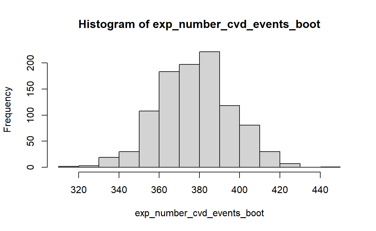
# Calculate mean
mean(exp_number_cvd_events_boot)
[1] 377.7711# Calculate standard deviation
sd(exp_number_cvd_events_boot)[1] 18.12974 2.5% 97.5%
340.0596 412.4694 Risk classification tool
### Build risk classification tool
cvd_risk_classification <- function(age_input = 50,
                                    gender_input = "female",
                                    smoking_input = "no",
                                    bmi_input = 25,
                                    systolic_bp_input = 130,
                                    diastolic_bp_input = 80){

  # Create hypertension indicator
   hypertension_input <- if_else(systolic_bp_input >= 140 | diastolic_bp_input >= 90, "yes", "no")

  # Create input dataframe
   data_new <- data.frame(age = c(age_input),
                          gender = c(gender_input),
                          smoking = c(smoking_input),
                          bmi = c(bmi_input),
                          hypertension = c(hypertension_input))

  # Calculate risk score
   risk_score <- predict(logit_mod_boot, newdata = data_new, type = "response")

  # Create recommendation variable
   recommendation <- if_else(risk_score > 0.1, "Offer Life Style Change Program", "No Action Needed")

  # Output recommendation
   print(recommendation)

}

### Check the functionality of the function
# Low risk applicant
cvd_risk_classification(age_input = 35,
                        gender_input = "female",
                        smoking_input = "no",
                        bmi_input = 23,
                        systolic_bp_input = 127,
                        diastolic_bp_input = 79)
[1] "No Action Needed"# High risk applicant
cvd_risk_classification(age_input = 57,
gender_input = "male",
smoking_input = "yes",
bmi_input = 31,
systolic_bp_input = 145,
diastolic_bp_input = 97)[1] "Offer Life Style Change Program"