Getting ready
Task 1
Create an R project for solving this Exercise Sheet.
Task 2
Download the csv-file SSRC_data.csv and the R script SSRC_C5_template.R and put it in the R project folder you created in Task 1.
Task 3
Open the SSRC_C6_template.R R Script.
Task 4
Load the tidyverse package.
# Load tidyverse package
library("tidyverse")
Task 5
Use the read.csv() command to load the SSRC data into R and call the respective data object SSRC_data.
# Load the dataset
SSRC_data <- read.csv("SSRC_data.csv")
Task 6
Get a first impression of the dataset by checking out the dataset using the str() command.
# Check out the dataset
str(SSRC_data)
'data.frame': 1000 obs. of 5 variables:
$ age : int 64 59 39 30 49 37 33 44 27 55 ...
$ gender : chr "male" "female" "female" "female" ...
$ education_level : chr "medium" "low" "high" "high" ...
$ physical_activity_level: chr "low" "medium" "low" "low" ...
$ bmi : num 27.9 27.5 27.4 24.2 23.9 30.7 25.1 30.3 18.5 30.2 ...Task 7
Transform the three categorical variables in the dataset into factor variables. Make sure that the levels of the physical_activity_level and education_level variables are ordered in a reasonable way.
# Transform into factor variables
SSRC_data <- mutate(SSRC_data, gender = as.factor(gender),
                               education_level = as.factor(education_level),
                               physical_activity_level = as.factor(physical_activity_level))

# Order education_level and physical_activity_level in a reasonable way
SSRC_data <- SSRC_data %>%
              mutate(education_level = fct_relevel(education_level, c("low", "medium", "high"))) %>%
              mutate(physical_activity_level = fct_relevel(physical_activity_level, c("low", "medium", "high")))

# Check whether it worked out
levels(SSRC_data$education_level)
[1] "low" "medium" "high" levels(SSRC_data$physical_activity_level)[1] "low" "medium" "high" Functions
Task 8
Estimate a linear regression model with bmi as dependent variable and all other variables in the SSRC data set as independent variables. Call this model lm_mod.
# Estimate the model
lm_mod <- lm(bmi ~ age + gender + education_level + physical_activity_level, data = SSRC_data)
Task 9
Create a data frame with one observation including the four variables: age, gender, education_level and physical_activity_level. The observation is a female person of age 45 who features a medium level of education and a medium level of physical activity. Call this data frame SSRC_data_new.
# Create data frame
SSRC_data_new <- data.frame(age = c(45),
                            gender = c("female"),
                            education_level = c("medium"),
                            physical_activity_level = c("medium"))
Task 10
Use the lm_mod model to predict the bmi for the new observation described in Task 9.
# Predict bmi for new observation
predict(object = lm_mod,
        newdata = SSRC_data_new)
1
25.81384 Task 11
Build a function that enables a convenient bmi prediction for a particular set of covariables.
The prediction should be based on the same model that you estimated in Task 8.
Arguments of the function should be a data frame called data_input (default: SSRC_data) and the four variables age_input (default: 45), gender_input (default:“female”), education_input (default: “medium”) and physical_input (default = “medium”).
Call the function bmi_pred_funct.
# Build the function
bmi_pred_funct <- function(data_input = SSRC_data,
                           age_input = 45,
                           gender_input = "female",
                           education_input = "medium",
                           physical_input = "medium"){

                    # Estimate model
                    lm_mod <- lm(bmi ~ age + gender + education_level + physical_activity_level,
                                 data = data_input)

                    # Set up data frame with new data
                    SSRC_data_new <- data.frame(age = c(age_input),
                                                gender = c(gender_input),
                                                education_level = c(education_input),
                                                physical_activity_level = c(physical_input))

                    # Predict bmi for the new data
                    bmi_prediction <- predict(object = lm_mod,
                                      newdata = SSRC_data_new)

                    # Return the prediction
                    return(bmi_prediction)

}
Task 12
Run the bmi_pred_funct function with its default values.
# Run the function
bmi_pred_funct()
1
25.81384 Task 13
Use the bmi_pred_funct function to predict the bmi of a male person of age 59 who features a low level of education and a low level of physical activity.
# Run the function
bmi_pred_funct(data_input = SSRC_data,
               age_input = 59,
               gender_input = "male",
               education_input = "low",
               physical_input = "low")
1
29.36972 Loops
Task 14
Use the bmi_pred_funct to predict the bmi for 5 female persons that are 20, 30, 40, 50 and 60 years old. All of them feature a medium education level and a medium physical activity level.
# Age 20
bmi_pred_funct(data_input = SSRC_data,
               age_input = 20,
               gender_input = "female",
               education_input = "medium",
               physical_input = "medium")
1
23.51512 # Age 30
bmi_pred_funct(data_input = SSRC_data,
age_input = 30,
gender_input = "female",
education_input = "medium",
physical_input = "medium") 1
24.43461 # Age 40
bmi_pred_funct(data_input = SSRC_data,
age_input = 40,
gender_input = "female",
education_input = "medium",
physical_input = "medium") 1
25.3541 # Age 50
bmi_pred_funct(data_input = SSRC_data,
age_input = 50,
gender_input = "female",
education_input = "medium",
physical_input = "medium") 1
26.27359 # Age 60
bmi_pred_funct(data_input = SSRC_data,
age_input = 60,
gender_input = "female",
education_input = "medium",
physical_input = "medium") 1
27.19308 Task 15
Do the exact same thing as in Task 14 but this time you should use a for loop to do so.
# Create age vector
age_vector <- c(20, 30, 40, 50, 60)
# Use for loop to make bmi predictions for each age in the age vector
for (i in 1:length(age_vector)){
print(
bmi_pred_funct(data_input = SSRC_data,
age_input = age_vector[i],
gender_input = "female",
education_input = "medium",
physical_input = "medium")
)
} 1
23.51512
       1
24.43461
      1
25.3541
       1
26.27359
       1
27.19308
Task 16
Do the exact same thing as in Task 15 but this time you save the results of each iteration in a vector called bmi_predictions. Check out the content of this vector after creating it.
# Create age vector
age_vector <- c(20, 30, 40, 50, 60)

# Create vector to store the results
bmi_predictions <- numeric(length(age_vector))

# Use for loop to make bmi predictions for each age and store it
for (i in 1:length(age_vector)){
          bmi_predictions[i] <- bmi_pred_funct(data_input = SSRC_data,
                                               age_input = age_vector[i],
                                               gender_input = "female",
                                               education_input = "medium",
                                               physical_input = "medium")

}

# Check out the vector
bmi_predictions
[1] 23.51512 24.43461 25.35410 26.27359 27.19308Bootstrap
In the following tasks we always focus on the bmi prediction for a person that features the default values of our bmi_pred_funct function. We call such a person “default person”.
Task 17
Use our bmi_pred_funct function to check out the prediction for our default person.
# Run the function
bmi_pred_funct()
1
25.81384 Task 18
Use the sample_n() command from the dplyr package to draw a random sample (n = 1000) with replacement from our original SSRC dataset. Call this sample SSRC_data_bootstrap.
# Create dataset
SSRC_data_bootstrap <- sample_n(SSRC_data, 1000, replace = TRUE)
Task 19
Apply bmi_pred_funct to the SSRC_data_bootstrap dataset to predict the bmi of our default person.
# Apply function to the bootstrap dataset
bmi_pred_funct(data_input = SSRC_data_bootstrap)
1
25.33084 Task 20
Use a for loop to repeat what you did in tasks 18/19 1000 times. Store the results in a vector called bmi_pred_boot. Check out the bmi_pred_boot vector.
# Create vector for the results
bmi_pred_boot <- numeric(1000)

# Use for loop to fill results vector
for (i in 1:length(bmi_pred_boot)){

      # Create dataset
      SSRC_data_bootstrap <- sample_n(SSRC_data, 1000, replace = TRUE)

      # Apply function to the bootstrap dataset and save it in the results vector
      bmi_pred_boot[i] <- bmi_pred_funct(data_input = SSRC_data_bootstrap)
}

# Check out the vector
head(bmi_pred_boot)
[1] 25.95836 25.75462 25.91827 25.85037 25.61350 25.63804Task 21
Create a histogram to analyse the distribution of bmi_pred_boot vector. (Just use hist() from the base R package)
# Create Histogram
hist(bmi_pred_boot)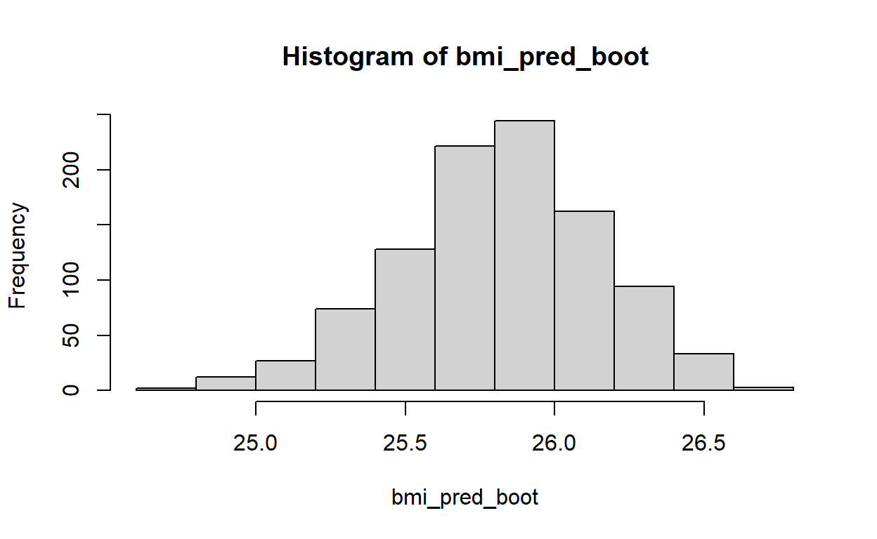
Task 22
Calculate the mean, standard deviation and the 0.025 and 0.975 quantiles for the bmi_pred_boot vector.
# Calculate mean
mean(bmi_pred_boot)
[1] 25.81372# Calculate standard deviation
sd(bmi_pred_boot)[1] 0.3359121 2.5% 97.5%
25.10069 26.46343